Book a Demo of MachineMetrics
The leading platform to collect, monitor, analyze, and drive action with machine data. Set up time with a product specialist to learn how we can help your operation.
Ready to empower your shop floor?
Learn More.svg)

In parts 1 and 2, we discussed the business problem and preprocessing involved with detecting anomalous behavior on machines. In this post, we’ll cover some creative data wrangling and clustering methods. This piece will be more technical in nature than the others.
Isolating Part Signatures and Creating Transformations
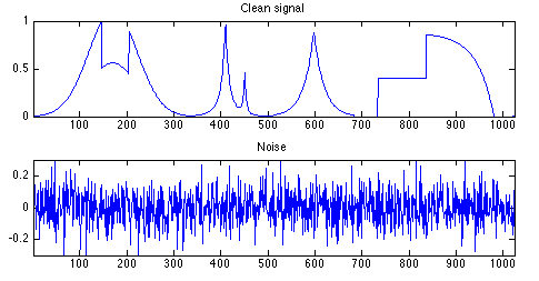
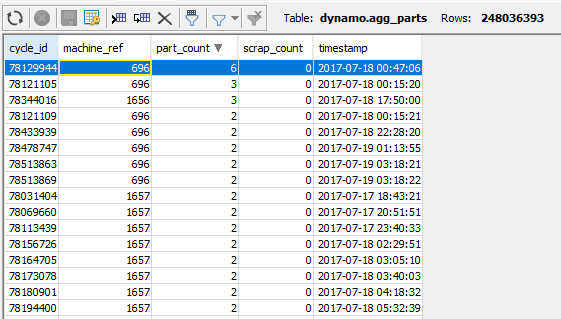
Once we have our clean signal, we need to split that signal up into its individual components, the part machining signature. Each part machining signature represents one part being made and the corresponding positions, feeds, speeds and loads which are attached to it.
We take each signature and line them up next to one another, creating a table where each ‘variable’ is a unique part being created and its affiliated data.
Determining Latent Structure of Part Signatures
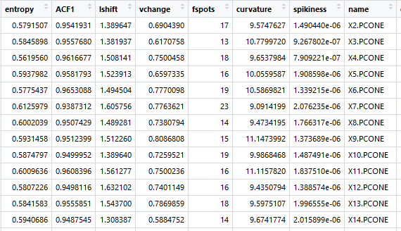
For our next step, we turn to Rob Hyndman and his anomalous package to detect the latent structure of each variable. The reasoning behind this is that each signature’s raw values are too volatile to be compared against one another, even when smoothing them out by taking rolling averages or other transformations. Thus, we must find another way to represent these signatures in a more stable manner. Hyndman determined several key metrics of time series which capture their inherent qualities. We select the most relevant ones for this use case, which are outlined below in non-technical terms. These are used to quantify the intrinsic factors of each part signature.
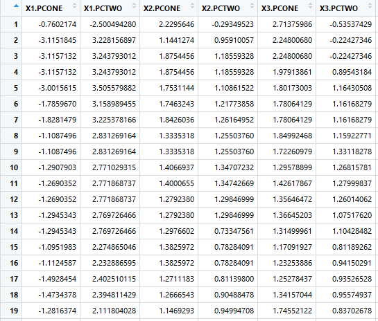
Each part signature is now represented by these seven dimensions. Anomalies are detected based on these attributes, which boil down the entire time series. The resultant table looks like the following, with each signature distilled down into these characteristics. Each part signature is one row.
Projecting Latent Features onto 2D plane Using PCA
Once we obtain these metrics, we apply PCA to these seven dimensions to reduce them down into two principal components. We then plot the two principal components in a 2D scatterplot.
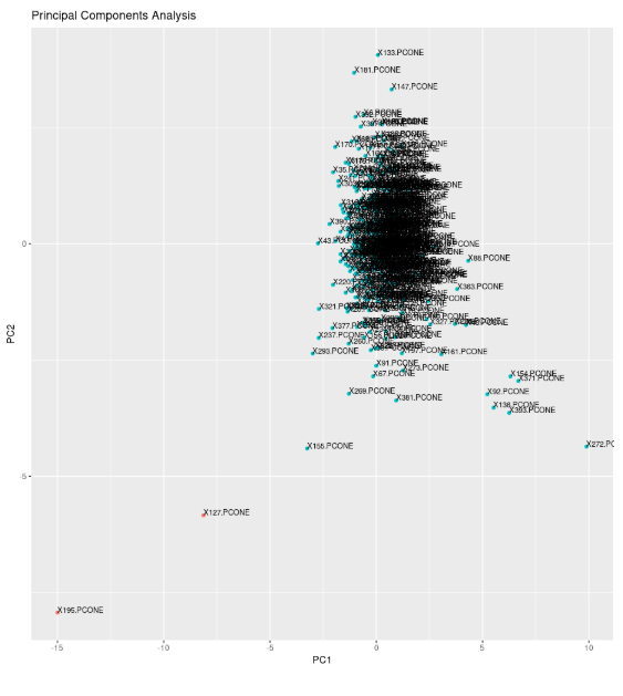
We can see just by eyeballing the plot above that there exists a central cluster of part signatures, with some scattered signatures on the outskirts and some way far off. The ones that are ‘way far off’ are our anomalies. The ones that are slightly far off may be capturing our measurement error, or are minor deviations from normal machining activity which may include scenarios like a slight deviation in load or spindle speed due to ambient conditions.
Why didn’t we take transformations?
It should also be noted that we tested several transformations of our data, including taking the log, rolling means, rolling standard deviation, and first derivative. We discovered that just taking the non-transformed signature is most effective way of detecting anomalies. We define most effective as separating out true anomalies most from the other points in 2D PCA space. This also makes sense theoretically, as
Using Clustering to Identify Outliers
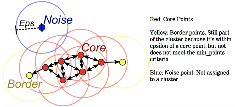
We can certainly eyeball outliers, but using clustering is a standardized way to determine when something is an outlier. We use an algorithm called DBSCAN which detects clusters by drawing a circle around each point and looking for other points in its neighborhood. DBSCAN requires two critical arguments — the “epsilon”, which is a circular region drawn around each point to determine cluster neighborhoods, and the “minimum points threshold”, which is the number of points that must fall in that neighborhood for it to be considered a cluster.
An illustration of DBSCAN is below. “Core” points are considered non-anomalous, “border” points, which are on the border of the circle are also non-anomalous. However, “noise” points which are outside the central region completely are anomalies.
Determining the epsilon
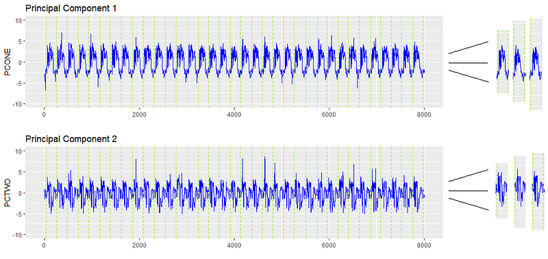
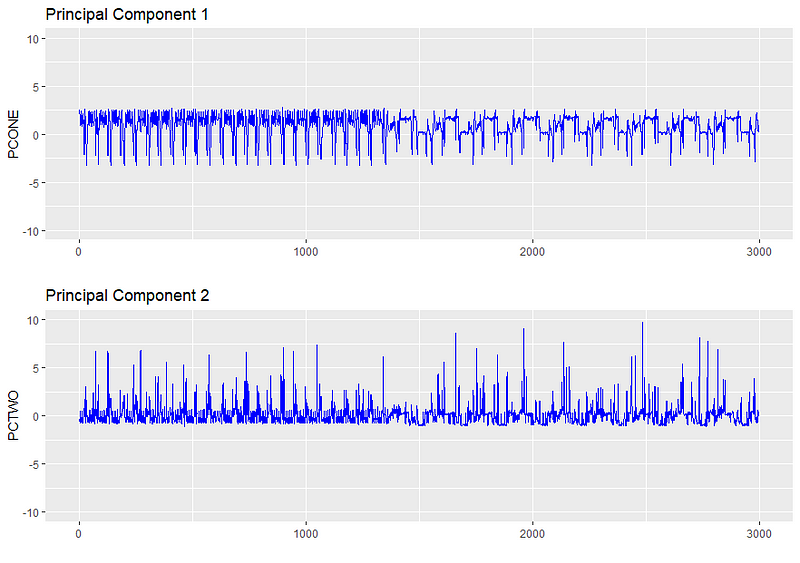
The tuning process required looking at the distribution of the data and selecting parameters which isolated a small minority of points, while not completely excluding anomalies. To get a rough order of magnitude of where epsilon should be, we plot distributions for Principal Component 1 and Principal Component 2, using this particular scenario as an example representative of most scenarios.
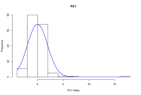
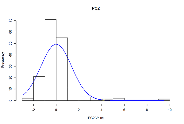
Due to the centering, the principal components are roughly normally distributed with a mean of zero and standard deviation of 1.5. In a normal distribution, 68% of observations are encompassed in one standard deviation, 95% in two, and 99.7% in three.
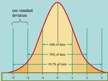
This means that given a 1.5 PC standard deviation, ~68% of the observations fall between -1.5 and 1.5 PCs, 95% fall between -3 and 3, and 99.7% fall between -4.5 and 4.5.
We know that excluding outlier machines, the average scrap rate for MachineMetrics customers, inclusive of human error, is ~1/1000 parts, which is a 99.9% success rate (MachineMetrics customers have collectively made 327 million parts, and 224k were scrapped). While this may seem high, we should keep in mind that our customers are mostly smaller machine shops that may not have huge volume of the same part being manufactured. Additionally, a large portion of our customers are job-shops, which manufacture ad-hoc, one off parts for other companies, giving them less time to perfect the manufacturing process and thus leaving more room for error.
In a normal distribution 99.9% of observations fall within 3 standard deviations, which in our case is ± 4.5 units in the principal component values. In consideration of the fact that precision (preventing false positives) is more important than recall (capturing all the anomalies) when first piloting this method, we set our epsilon threshold to be 4 standard deviations away, i.e. points must fall 6 units away from the central cluster to be considered an outlier. We consider precision more important because customers may choose to ignore the notifications if too many are given, and we want to avoid creating unnecessary panic*.
*this part is still in pilot and parameters are subject to change
Determining the minimum points threshold
The minimum points threshold sets the minimum number of points that must be clustered together in order for it to be considered its own independent cluster, rather than just outlier points. This can be useful in circumstances where there’s not actually an outlier, but rather periods with tooling changes or other systemic but normal differences. In these cases, the machine may reset itself to a normal state within a short span of time. We define this threshold to be 10 points.
We thus define a cluster to have a minimum of ten points, and the size of the epsilon radius to be 6 units. Anything that falls past 6 units of the main cloud, and has less than 10 points near it is an anomaly. In this case, we have detected two anomalies, corresponding to two parts that had ‘outlier’ machining signatures. We can identify when these parts are made, and code the times corresponding to them as times when the machine was exhibiting anomalous behavior.
Verifying an anomalous part
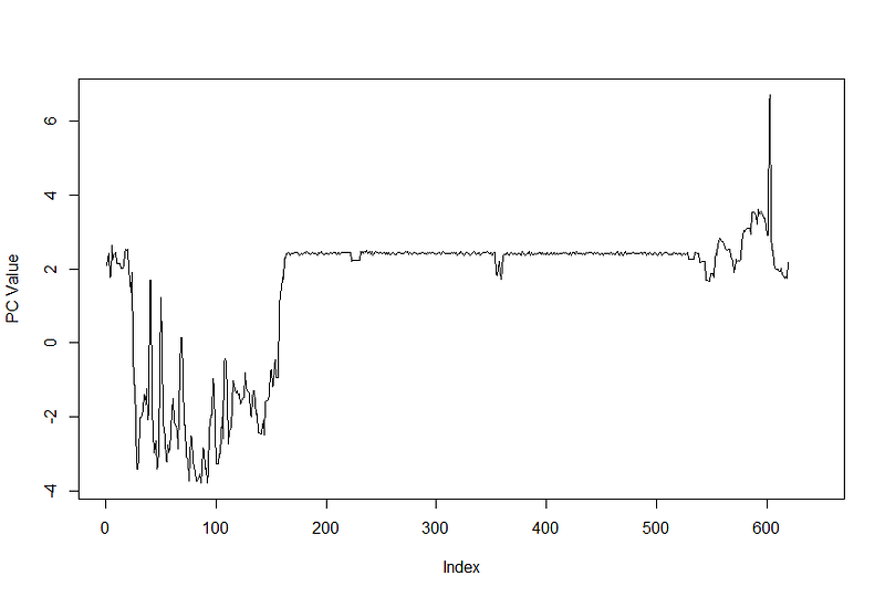
Part 127 was detected to be anomalous, which was created between 3:04 and 3:07 AM. Let’s take a look at what the signature looks like.

As we can see, there was clearly a difference in the part signature. In this circumstance, the machine hung for a few minutes, reset itself, then continued machining activity. Though there was no immediate consequence this time, the operator was alerted to this and took further steps to investigate unexpected hangs, as it could result in tool failure in the future.
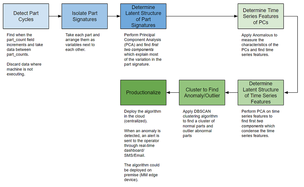
Summary of Steps
We’ve covered alot in the last few blog posts. To help summarize everything, a flow chart is provided below for easier understanding of the process. In the last part of our series, we’ll cover productionalization.
Alternative Use Case
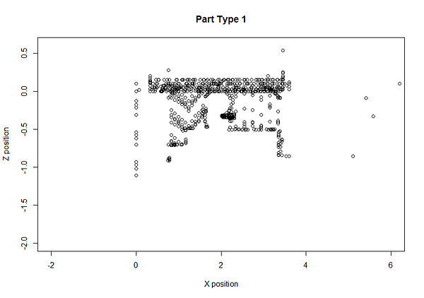
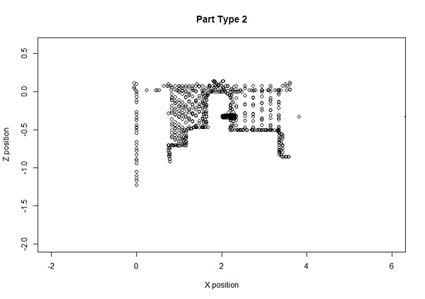
An alternative use for this method is detecting when the part being manufactured changed. Using the same steps, and adjusting the epsilon to be more appropriate for the situation, we can detect when the part signatures look structurally different and form another cluster. In the example below, we can see that there was a part change at Part 62 (that part itself is anomalous due to the actual changeover process, but we can add extra rules to exclude anomalies). The green cloud is one type of part, and the blue cloud another. This lets us automatically categorize parts that the customer has made.
We can look back and see that the characteristics of the part signatures do indeed see a significant shift when a new part type is made.
We verified against ground-truth data in our database and confirmed there was a new type of part manufactured at this time. Since MachineMetrics tracks and stores tool positions, we can even plot the part to ascertain this.
Ready to empower your shop floor?
Learn More

.png?width=1960&height=1300&name=01_comp_Downtime-%26-Quality_laptop%20(1).png)
Comments