
Book a Demo of MachineMetrics
The leading platform to collect, monitor, analyze, and drive action with machine data. Set up time with a product specialist to learn how we can help your operation.
Ready to empower your shop floor?
Learn More.svg)

In the last post of this series, we went over why it was important to try and detect anomalous behavior on machines. In this post, we’ll dive right into how we preprocessed and cleaned the data.
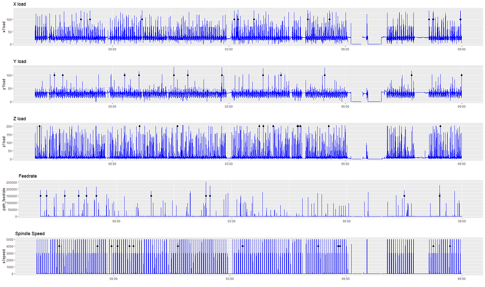
We tried this method on many machines, but to illustrate our points, we’ll single out just one example. We’ll begin by looking at what the machining process looks like from our standpoint. Below we plot streaming data for feeds, speeds, and load for one particular machine from 10 PM to 9 AM. This machine is making the same part the whole time.

We can see that the data is noisy — we don’t know what’s relevant to look at, nor what we’re looking for in terms of anomalies. Why are the signals so irregular and spiky, and why are there gaps in the signals? If the machine is making the same part, why is there seemingly little regularity to the signals?
This is because of the way MachineMetrics collects data. Every 900 ms or so, we open a “window” to detect changes in the metrics. If there is a change, we record it. If not, we don’t record anything. We do this for two main reasons:
Metrics almost certainly change more than every 900 ms, which means the exact same part being manufactured can look different based on when the window is open. For the solution to this problem, we need to leverage our domain knowledge and some hardcore data cleaning to get to a usable signal.
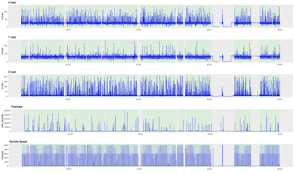
If we try and apply anomaly detection to these signals as they are without cleaning them, the anomalies picked up are not meaningful. We run our time-series through the anomalize package and plot the results below. Anomalize performs single-stream anomaly detection. Anomalies appear as black dots, which can occur at different times in different signals.
Though some of these signals may look like outliers to the naked eye, the anomalies detected are not in fact useful. They do not give an indication of truly unusual behavior, as they’re more an artifact of our data collection process. So, it’s time to get our hands dirty with the data. First, we’ll tackle the issue of downtime (gaps). Then, we’ll get to how we smoothed over the sampling frequency issue.
Removing Inactive Sequences
Mixed in with this data is lots of downtime. This downtime includes operator downtime (3 am snack, shift changes), and machine downtime (built-in cooling time, tool changes, and in this case, two anomalies which we’ll decode).
Our first step is to find out when parts are created and how long it takes to make a part. We don’t really care that there may have been regular tool changes when the machine wasn’t actively working, and we don’t want our algorithm to pick this up as an anomaly during the machining process.
Our first step is to filter out the signal (sequences we care about), vs. the noise (sequences that are irrelevant). We also want to make sure we don’t exclude truly anomalous behavior from the data.
To make this easier, MachineMetrics collects a “part_count” field, which increments whenever a part is finished being machined. We capture this field through tapping into two key components of the machine:
2. In other types, we can tap into the programmable logic control (PLC) of the machine, which includes a signal in the G-code (CNC programming language) that indicates part completion.
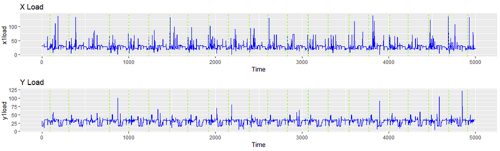
Let’s superimpose part_count on the previous visualization to see what the part creation cycles look like. Each dotted green line represents the creation of one part.
MachineMetrics also collects a “machine status” field from the control, which indicates if the machine is actively machining or not. Again, this is collected by tapping into the relays or the control.
We only want to preserve observations where the machine is active. In the plot below, red indicates regions where the machine was inactive (or in setup, etc.) and where we eliminated observations.
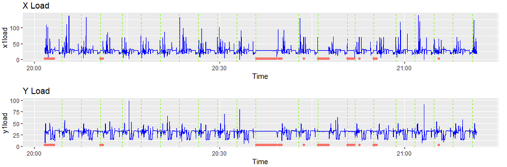
After being cleaned, the signal looks like the following. Note the change in timescale as removing observations in the time-series transforms it into a vector.
The signal now looks much neater, resembling typical signal data like vibration, speech or power. This is significant because anomaly detection methods have previously been applied to those types of signals, and generating an analog to these signals expands our repertoire of methodologies.
Detecting Latent Structure of Machining Process
After gathering feedback from machinist interviews, the relationship between loads, positions, spindle speeds, and feedrate is often the critical factor to look at. For example, it’s not relevant if speeds, feeds, and load all fall to zero at the same time — this may merely indicate the machine is resting. It’s a problem however if the machine continues to feed the material but loads fall to zero, signifying a deeper issue at hand. Or, if the position of the axes continue on their regular path but there is no more load associated with it, this could mean the tool bit broke off.

It turns out that despite the window measurement error, the relationships largely remain the same across normal part signatures due to the number of observations involved. Over time, normal parts will have similar signatures, though the range of what signatures look like will be larger.
We need to find a meaningful way to measure the correlations or relationships between all these signals and distill them into one or two combined signals, encompassing all feeds, speeds, loads and positions.
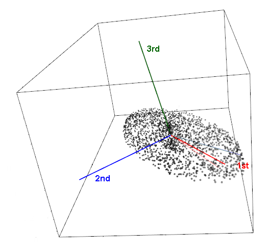
We look to a method called Principal Components Analysis (PCA) to distill our many signals into two signals that are representative of all of them. PCA takes a multi-dimensional matrix and distills it into its ‘principal components’ by capturing the direction of most variance. For example, if 70% of the variance of your data set can be captured in one dimension, and 95% can be captured in two dimensions, we only lose 5% of the information in our data by eliminating all the other variables. Intuitively, it keeps combinations of the variables that can represent the data the best, and meaning can often be derived from these combined variables as the implied information underpinning your data set.
For example, a dataset may have four variables — Industrial Production, Crime Rate, Consumer Price Index, and an Income Inequality Index for each country. PCA may determine two principal components capture almost all the information, the first being a combination of Industrial Production and Consumer Price Index, basically representing GDP (the implied variable underpinning both), and the second being a combo of Crime Rate and Income Inequality (the implied variable representing something akin to social unrest).
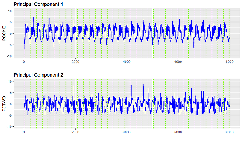
In our case, the multi-dimensional matrix is the collection of all positions, feeds, speeds, and loads (33 variables for this machine). We reduce all these variables into two principal components which capture the important information from the 33 original variables. We are able to identify decouplings of relationships, as the values in the principal signals will be sensitive to when unusual relationships arise between the original 33.

After finding the latent signals, we can plot them and see that there is in fact quite a consistent signal. With this cleaned signal, we can start performing more of the heavy lifting of anomaly detection.
Ready to empower your shop floor?
Learn More

.png?width=1960&height=1300&name=01_comp_Downtime-%26-Quality_laptop%20(1).png)


Comments